Seeding, transduction, out-of-sample error and the Microsoft approach...

My past master's student Adam Teichert (now at JHU) did some work on inducing part of speech taggers using typological information.  We wanted to compare the usefulness of using small amounts of linguistic information with small amounts of lexical information in the form of seeds.  (Other papers give seeds different names, like initial dictionaries or prototypes or whatever... it's all the same basic idea.)

The basic result was that if you don't use seeds, then typological information can help a lot.  If you do you seeds, then your baseline performance jumps from like 5% to about 40% and then using typological information on top of this isn't really that beneficial.

This was a bit frustrating, and led us to think more about the problem.  The way we got seeds was to look at the wikipedia page about Portuguese (for instance) and use their example list of words for each tag.  An alternative popular way is to use labeled data and extract the few most frequent words for each part of speech type.  They're not identical, but there is definitely quite a bit of overlap between the words that Wikipedia lists as examples of determiners and the most frequent determiners (this correlation is especially strong for closed-class words).

In terms of end performance, there are two reasons seeds can help.  The first, which is the interesting case, is that knowing that "the" is a determiner helps you find other determiners (like "a") and perhaps also nouns (for instance, knowing the determiners often precede nouns in Portuguese).  The second, which is the uninteresting case, is that now every time you see one of your seeds, you pretty much always get it right.  In other words, just by specifying seeds, especially by frequency (or approximately by frequency ala Wikipedia), you're basically ensuring that you get 90% accuracy (due to ambiguity) on some large fraction of the corpus (again, especially for closed-class words which have short tails).

This phenomena is mentioned in the text (but not the tables :P), for instance, in Haghighi & Klein's 2006 NAACL paper on prototype-driven POS tagging, wherein they say: "Adding prototypes ... gave an accuracy of 68.8% on all tokens, but only 47.7% on non-prototype occurrences, which is only a marginal improvement over [a baseline system with no prototypes."  Their improved system remedies this and achieves better accuracy on non-prototypes as well as prototypes (aka seeds).

This is very similar to the idea of transductive learning in machine learning land.  Transduction is an alternative to semi-supervised learning.  The setting is that you get a bunch of data, some of which is labeled and some of which is unlabeled.  Your goal is to simply label the unlabeled data.  You need not "induce" the labeling function (though many approach do, in passing).

The interesting thing is that learning with seeds is very similar to transductive learning, though perhaps with a bit stronger assumption of noise on the "labeled" part.  The irony is that in machine learning land, you would never report "combined training and test accuracy" -- this would be ridiculous.  Yet this is what we seem to like to do in NLP land.  This is itself related to an old idea in machine learning wherein you rate yourself only on test example that you didn't see at training time.  This is your out-of-sample error, and is obviously much harder than your standard generalization error.  (The famous no-free-lunch theorems are from an out-of-sample analysis.)  The funny thing out of sample error is that sometimes you prefer not to get more training examples, because you then know you won't be tested on it!  If you were getting it right already, this just hurts you.  (Perhaps you should be allowed to see x and say "no I don't want to see y"?)

I think the key question is: what are we trying to do.  If we're trying to build good taggers (i.e., we're engineers) then overall accuracy is what we care about and including "seed" performance in our evaluations make sense.  But when we're talking about 45% tagging accuracy (like Adam and I were), then this is a pretty pathetic claim.  In the case that we're trying to understand learning algorithms and study their performance on real data (i.e., we're scientists) then accuracy on non-seeds is perhaps more interesting.  (Please don't jump on me for the engineer/scientist distinction: it's obviously much more subtle than this.)

This also reminds me of something Eric Brill said to me when I was working with him as a summer intern in MLAS at Microsoft (back when MLAS existed and back when Eric was in MLAS....).  We were working on web search stuff.  His comment was that he really didn't care about doing well on the 1000 most frequent queries.  Microsoft could always hire a couple annotators to manually do a good job on these queries.  And in fact, this is what is often done.  What we care about is the heavy tail, where there are too many somewhat common things to have humans annotate them all.  This is precisely the same situation here.  I can easily get 1000 seeds for a new language.  Do I actually care how well I do on those, or do I care how well I do on the other 20000+ things?

Comparing Bounds

This is something that's bothered me for quite a while, and I don't know of a good answer.  I used to think it was something that theory people didn't worry about, but then this exact issue was brought up by a reviewer of a theory-heavy paper that we have at NIPS this year (with Avishek Saha and Abhishek Kumar). There are (at least?) two issues with comparing bounds, the first is the obvious "these are both upper bounds, what does it mean to compare them?"  The second is the slightly less obvious "but your empirical losses may be totally different" issue.  It's actually the second one that I want to talk about, but I have much less of a good internal feel about it.

Let's say that I'm considering two learning approaches.  Say it's SVMs versus logistic regression.  Both regularized.  Or something.  Doesn't really matter.  At the end of the day, I'll have a bound that looks roughly like:

        expected test error <= empirical training error + f( complexity / N)

Here, f is often "sqrt", but could really be any function.  And N is the number of data points.

Between two algorithms, both "f" and "complexity" can vary.  For instance, one might have a linear dependence on the dimensionality of the data (i.e., complexity looks like O(D), where D is dimensionality) and the other might have a superlinear dependence (eg., O(D log D)).  Or one might have a square root.  Who knows.  Sometimes there's an inf or sup hiding in there, too, for instance in a lot of the margin bounds.

At the end of the day, we of course want to say "my algorithm is better than your algorithm."  (What else is there in life?)  The standard way to say this is that "my f(complexity / N) looks better than your f'(complexity' / N)."

Here's where two issues crop up.  The first is that our bound is just an upper bound.  For instance, Alice could come up to me and say "I'm thinking of a number between 1 and 10" and Bob could say "I'm thinking of a number between 1 and 100."  Even though the bound is lower for Alice, it doesn't mean that Alice is actually thinking of a smaller number -- maybe Alice is thinking of 9 and Bob of 5.  In this way, the bounds can be misleading.

My general approach with this issue is to squint, as I do for experimental results.  I don't actually care about constant factors: I just care about things like "what does the dependence on D look like."  Since D is usually huge for problems I care about, a linear or sublinear dependence on D looks really good to me.  Beyond that I don't really care.  I especially don't care if the proof techniques are quite similar.  For instance, if they both use Rademacher complexities, then I'm more willing to compare them than if one uses Rademacher complexities and the other uses covering numbers.  They somehow feel more comparable: I'm less likely to believe that the differences are due to the method of analysis.

(You can also get around this issue with some techniques, like Rademacher complexities, which give you both upper and lower bounds, but I don't think anyone really does that...)

The other issue I don't have as good a feeling for.  The issue is that we're entirely ignoring the "empirical training error" question.  In fact, this is often measured differently between different algorithms!  For instance, for SVMs, the formal statement is more like "expected 0/1 loss on test <= empirical hinge loss on training + ..."  Whereas for logistic regression, you might be comparing expected 0/1 loss with empirical log loss.

Now I really don't know what to do.

We ran into this issue because we were trying to compare some bounds between EasyAdapt and a simple model trained just on source data.  The problem is that the source training error might be totally incomparable to the (source + target) training error.

But the issue is for sure more general.  For instance, what if your training error is measured in squared error?  Now this can be huge when hinge loss is still rather small.  In fact, your squared error could be quadratically large in your hinge loss.  Actually it could be arbitrarily larger, since hinge goes to zero for any sufficiently correct classification, but squared error does not.  (Neither does log loss.)

This worries me greatly, much more than the issue of comparing upper bounds.

Does this bother everyone, or is it just me?  Is there a good way to think about this that gets your out of this conundrum?

Manifold Assumption versus Margin Assumption

[This post is based on some discussions that came up while talking about manifold learning with Ross Whitaker and Sam Gerber, who had a great manifold learning paper at ICCV last year.]

There are two assumptions that are often used in statistical learning (both theory and practice, though probably more of the latter), especially in the semi-supervised setting.  Unfortunately, they're incompatible.

The margin assumption states that your data are well separated.  Usually it's in reference to linear, possibly kernelized, classifiers, but that need not be the case.  As most of us know, there are lots of other assumptions that boil down to the same thing, such as the low-weight-norm assumption, or the Gaussian prior assumption.  At the end of the day, it means your data looks like what you have on the left, below, not what you have on the right.

The manifold assumption that is particularly popular in semi-supervised learning, but also shows up in supervised learning, says that your data lie on a low dimensional manifold embedded in a higher dimensional space.  One way of thinking about this is saying that your features cannot covary arbitrarily, but the manifold assumption is quite a bit stronger.  It usually assumes a Reimannian (i.e., locally Euclidean) structure, with data points "sufficiently" densely sampled.  In other words, life looks like the left, not the right, below:

Okay, yes, I know that the "Bad" one is a 2D manifold embedded in 2D, but that's only because I can't draw 3D images :).  And anyway, this is a "weird" manifold in the sense that at one point (where the +s and -s meet), it drops down to 1D.  This is fine in math-manifold land, but usually not at all accounted for in ML-manifold land.

The problem, of course, is that once you say "margin" and "manifold" in the same sentence, things just can't possibly work out.  You'd end up with a picture like:

This is fine from a margin perspective, but it's definitely not a (densely sampled) manifold any more.

In fact, almost by definition, once you stick a margin into a manifold (which is okay, since you'll define margin Euclideanly, and manifolds know how to deal with Euclidean geometry locally), you're hosed.

So I guess the question is: who do you believe?

Online Learning Algorithms that Work Harder

It seems to be a general goal in practical online learning algorithm development to have the updates be very very simply.  Perceptron is probably the simplest, and involves just a few adds.  Winnow takes a few multiplies.  MIRA takes a bit more, but still nothing hugely complicated.  Same with stochastic gradient descent algorithms for, eg., hinge loss.

I think this maybe used to make sense.  I'm not sure that it makes sense any more.  In particular, I would be happier with online algorithms that do more work per data point, but require only one pass over the data.  There are really only two examples I know of: the StreamSVM work that my student Piyush did with me and Suresh, and the confidence-weighted work by Mark Dredze, Koby Crammer and Fernando Pereira (note that they maybe weren't trying to make a one-pass algorithm, but it does seem to work well in that setting).

Why do I feel this way?

Well, if you look even at standard classification tasks, you'll find that if you have a highly optimized, dual threaded implementation of stochastic gradient descent, then your bottleneck becomes I/O, not learning.  This is what John Langford observed in his Vowpal Wabbit implementation.  He has to do multiple passes.  He deals with the I/O bottleneck by creating an I/O friendly, proprietary version of the input file during the first past, and then careening through it on subsequent passes.

In this case, basically what John is seeing is that I/O is too slow.  Or, phrased differently, learning is too fast :).  I never thought I'd say that, but I think it's true.  Especially when you consider that just having two threads is a pretty low requirement these days, it would be nice to put 8 or 16 threads to good use.

But I think the problem is actually quite a bit more severe.  You can tell this by realizing that the idealized world in which binary classifier algorithms usually get developed is, well, idealized.  In particular, someone has already gone through the effort of computing all your features for you.  Even running something simple like a tokenizer, stemmer and stop word remover over documents takes a non-negligible amount of time (to convince yourself: run it over Gigaword and see how long it takes!), easily much longer than a silly perceptron update.

So in the real world, you're probably going to be computing your features and learning on the fly.  (Or at least that's what I always do.)  In which case, if you have a few threads computing features and one thread learning, your learning thread is always going to be stalling, waiting for features.

One way to partially circumvent this is to do a variant of what John does: create a big scratch file as you go and write everything to this file on the first pass, so you can just read from it on subsequent passes.  In fact, I believe this is what Ryan McDonald does in MSTParser (he can correct me in the comments if I'm wrong :P).  I've never tried this myself because I am lazy.  Plus, it adds unnecessary complexity to your code, requires you to chew up disk, and of course adds its own delays since you now have to be writing to disk (which gives you tons of seeks to go back to where you were reading from initially).

A similar problem crops up in structured problems.  Since you usually have to run inference to get a gradient, you end up spending way more time on your inference than your gradients.  (This is similar to the problems you run into when trying to parallelize the structured perceptron.)

Anyway, at the end of the day, I would probably be happier with an online algorithm that spent a little more energy per-example and required fewer passes; I hope someone will invent one for me!

Finite State NLP with Unlabeled Data on Both Sides

(Can you tell, by the recent frequency of posts, that I'm try not to work on getting ready for classes next week?)

[This post is based partially on some conversations with Kevin Duh, though not in the finite state models formalism.]

The finite state machine approach to NLP is very appealing (I mean both string and tree automata) because you get to build little things in isolation and then chain them together in cool ways. Kevin Knight has a great slide about how to put these things together that I can't seem to find right now, but trust me that it's awesome, especially when he explains it to you :).

The other thing that's cool about them is that because you get to build them in isolation, you can use different data sets, which means data sets with different assumptions about the existence of "labels", to build each part. For instance, to do speech to speech transliteration from English to Japanese, you might build a component system like:

English speech --A--> English phonemes --B--> Japanese phonemes --C--> Japanese speech --D--> Japanese speech LM

You'll need a language model (D) for Japanese speech, that can be trained just on acoustic Japanese signals, then parallel Japanese speech/phonemes (for C), parallel English speech/phonemes (for A) and parallel English phonemes/Japanese phonemes (for B). [Plus, of course, if you're missing any of these, EM comes to your rescue!]

Let's take a simpler example, though the point I want to make applies to long chains, too.

Suppose I want to just do translation from French to English. I build an English language model (off of monolingual English text) and then an English-to-French transducer (remember that in the noisy channel, things flip direction). For the E2F transducer, I'll need parallel English/French text, of course. The English LM gives me p(e) and the transducer gives me p(f|e), which I can put together via Bayes' rule to get something proportional to p(e|f), which will let me translate new sentences.

But, presumably, I also have lots of monolingual French text. Forgetting math for a moment, which seems to suggest that this can't help me, we can ask: why should this help?

Well, it probably won't help with my English language model, but it should be able to help with my transducer. Why? Because my transducer is supposed to give me p(f|e). If I have some French sentence in my GigaFrench corpus to which my transducer assigns zero probability (for instance, max_e p(f|e) = 0), then this is probably a sign that something bad is happening.

More generally, I feel like the following two operations should probably give roughly the same probabilities:

1. Drawing an English sentence from the language model p(e).
2. Picking a French sentence at random from GigaFrench, and drawing an English sentence from p(e|f), where p(e|f) is the composition of the English LM and the transducer.

If you buy this, then perhaps one thing you could do is to try to learn a transducer q(f|e) that has low KL divergence between 1 and 2, above. If you work through the (short) make, and throw away terms that are independent of the transducer, then you end up wanting to minimize [ sum_e p(e) log sum_f q(f|e) ]. Here, the sum over f is a finite sum over GigaFrench, and the sum over e is an infinite sum over positive probability English sentences given my the English LM p(e).

One could then apply something like posterior regularization (Kuzman Ganchev, Graça and Taskar) to do the learning. There's the nasty bit about how to compute these things, but that's why you get to be friends with Jason Eisner so he can tell you how to do anything you could ever want to do with finite state models.

Anyway, it seems like an interesting idea. I'm definitely not aware if anyone has tried it.

Multi-task learning: should our hypothesis classes be the same?

It is almost an unspoken assumption in multitask learning (and domain adaptation) that you use the same type of classifier (or, more formally, the same hypothesis class) for all tasks. In NLP-land, this usually means that everything is a linear classifier, and the feature sets are the same for all tasks; in ML-land, this usually means that the same kernel is used for every task. In neural-networks land (ala Rich Caruana), this is enforced by the symmetric structure of the networks used.

I probably would have gone on not even considering this unspoken assumption, until a few years ago I saw a couple papers that challenged it, albeit indirectly. One was Factorizing Complex Models: A Case Study in Mention Detection by Radu (Hans) Florian, Hongyan Jing, Nanda Kambhatla and Imed Zitouni, all from IBM. They're actually considering solving tasks separately rather than jointly, but joint learning and multi-task learning are very closely related. What they see is that different features are useful for spotting entity spans, and for labeling entity types.

That year, or the next, I saw another paper (can't remember who or what -- if someone knows what I'm talking about, please comment!) that basically showed a similar thing, where a linear kernel was doing best for spotting entity spans, and a polynomial kernel was doing best for labeling the entity types (with the same feature sets, if I recall correctly).

Now, to some degree this is not surprising. If I put on my feature engineering hat, then I probably would design slightly different features for these two tasks. On the other hand, coming from a multitask learning perspective, this is surprising: if I believe that these tasks are related, shouldn't I also believe that I can do well solving them in the same hypothesis space?

This raises an important (IMO) question: if I want to allow my hypothesis classes to be different, what can I do?

One way is to punt: you can just concatenate your feature vectors and cross your fingers. Or, more nuanced, you can have some set of shared features and some set of features unique to each task. This is similar (the nuanced version, not the punting version) to what Jenny Finkel and Chris Manning did in their ACL paper this year, Hierarchical Joint Learning: Improving Joint Parsing and Named Entity Recognition with Non-Jointly Labeled Data.

An alternative approach is to let the two classifiers "talk" via unlabeled data. Although motivated differently, this was something of the idea behind my EMNLP 2008 paper on Cross-Task Knowledge-Constrained Self Training, where we run two models on unlabeled data and look for where they "agree."

A final idea that comes to mind, though I don't know if anyone has tried anything like this, would be to try to do some feature extraction over the two data sets. That is, basically think of it as a combination of multi-view learning (since we have two different hypothesis classes) and multi-task learning. Under the assumption that we have access to examples labeled for both tasks simultaneously (i.e., not the settings for either Jenny's paper or my paper), then one could do a 4-way kernel CCA, where data points are represented in terms of their task-1 kernel, task-2 kernel, task-1 label and task-2 label. This would be sort of a blending of CCA-for-multiview-learning and CCA-for-multi-task learning.

I'm not sure what the right way to go about this is, but I think it's something important to consider, especially since it's an assumption that usually goes unstated, even though empirical evidence seems to suggest it's not (always) the right assumption.

How I teach machine learning

I've had discussions about this with tons of people, and it seems like my approach is fairly odd. So I thought I'd blog about it because I've put a lot of thought into it over the past four offerings of the machine learning course here at Utah.

At a high level, if there is one thing I want them to remember after the semester is over it's the idea of generalization and how it relates to function complexity. That's it. Now, more operationally, I'd like them to learn SVMs (and kernels) and EM for generative models.

In my opinion, the whole tenor of the class is set by how it starts. Here's how I start.

1. Decision trees. No entropy. No mutual information. Just decision trees based on classification accuracy. Why? Because the point isn't to teach them decision trees. The point is to get as quickly as possible to the point where we can talk about things like generalization and function complexity. Why decision trees? Because EVERYONE gets them. They're so intuitive. And analogies to 20 questions abound. We also talk about the who notion of data being drawn from a distribution and what it means to predict well in the future.
   
   
2. Nearest neighbor classifiers. No radial basis functions, no locally weighted methods, etc. Why? Because I want to introduce the idea of thinking of data as points in high dimensional space. This is a big step for a lot of people, and one that takes some getting used to. We then do k-nearest neighbor and relate it to generalization, overfitting, etc. The punch line of this section is the idea of a decision boundary and the complexity of decision boundaries.
   
   
3. Linear algebra and calculus review. At this point, they're ready to see why these things matter. We've already hinted at learning as some sort of optimization (via decision trees) and data in high dimensions, hence calculus and linear algebra. Note: no real probability here.
   
   
4. Linear classifiers as methods for directly optimizing a decision boundary. We start with 0-1 loss and then move to perceptron. Students love perceptron because it's so procedural.
   

The rest follows mostly as almost every other machine learning course out there. But IMO these first four days are crucial. I've tried (in the past) starting with linear regression or linear classification and it's just a disaster. You spend too much time talking about unimportant stuff. The intro with error-based decision trees moving to kNN is amazingly useful.

The sad thing is that there are basically no books that follow any order even remotely like this. Except...drum roll... it's actually not far from what Mitchell's book does. Except he does kNN much later. It's really depressing how bad most machine learning books are from a pedagogical perspective... you'd think that in 12 years someone would have written something that works better.

On top of that, the most recent time I taught ML, I structured everything around recommender systems. You can actually make it all work, and it's a lot of fun. We actually did recommender systems for classes here at the U (I had about 90-odd students from AI the previous semester fill out ratings on classes they'd taken in the past). The data was a bit sparse, but I think it was a lot of fun.

The other thing I change most recently that I'm very happy with is that I have a full project on feature engineering. (It ties in to the course recommender system idea.) Why? Because most people who take ML, if they ever use it at all, will need to do this. It's maybe one of the most important things that they'll have to learn. We should try to teach it. Again, something that no one ever talks about in books.

Anyway, that's my set of tricks. If you have some that you particularly like, feel free to share!

When Maximum Likelihood Doesn't Make Sense

One of the most fun AHA moments in ML or stats is when you see that for multinomial distributions, your naive idea of relative frequency corresponds (through a bunch of calculus) to maximum likelihood estimation. Ditto means of Gaussians, though that's never quite as amazing because Gaussians seems sort of odd beasts anyway. It's nice when our intuitions match what stats tells us.

I'll often watch a DVD, and then leave it in the DVD player until I want to watch something else. Usually it will return to the menu screen and the timer display will go through 0:00, 0:01, 0:02, ..., until it hits the length of the title screen loop, and then go back to 0:00. What I always wonder when I glance up at it is "what is the actual length of the title screen loop?" That is, what is the highest value it'll count up to.

Being a good statistician, I set up a model. First I play the frequentist game. Since I glance up and pretty arbitrary times, my observations can be modeled as a uniform random variable from 0 to some upper bound U, which is the quantity I want to infer.

Supposing that I only make one observation, say 0:27, I want a maximum likelihood estimate of U. It's easy to see that U=27 is the maximum likelihood solution. Anything less than 27 will render my observation impossible. For any U>=27, my observation has probability 1/(U+1), so the ML solution is precisely U=27. Note that even if I observe five observations a <= b <= c <= d <= e, the ML solution is still U=e. Huh. The math works. The model is as correct as I could really imagine it. But this answer doesn't really seem reasonable to me. Somehow I expect a number greater than my observation to come about.

Perhaps I need a prior. That'll solve it. I'll add a prior p(U) and then do maximum a posteriori. Well, it's easy to see that if p(U) is unimodal, and its mode is less than my (highest) observation, then the MAP solution will still be the (highest) observation. If it's mode is more than my (highest) observation, then the MAP solution will be the mode of p(U). If I think about this a bit, it's hard for me to justify a multi-modal p(U), and also hard for me to be happy with a system in which my prior essentially completely determines my solution.

Or I could be fully Bayesian and look at a posterior distribution p(U | data). This will just be a left-truncated version of my prior, again, not very satisfying.

(Note that the "Maximum Likelihood Sets" idea, which I also like quite a bit, doesn't fix this problem either.)

It also really bugs me that only my largest observation really affects the answer. If I get one hundred observations, most of them centered around 0:10, and then one at 0:30, then I'd guess that 0:30 or 0:31 or 0:32 is probably the right answer. But if I observe a bunch of stuff spread roughly uniformly between 0:00 and 0:30, then I'd be more willing to believe something larger.

I don't really have a solution to this dilemma. Perhaps you could argue that my difficulties arise from the use of a Uniform distribution -- namely, that were I to use another distribution, these problems wouldn't really arise. I don't think this is quite true, as described below:

We actually run in to this problem in NLP fairly often. I observe a billion documents and see, in this 1b documents, 100k unique words, many of which are singletons. But I'm not willing to believe that if I see that document 1,000,000,001, that there won't be a new unseen word. Sure it's less likely that I see a new unique word than in document 1001, where it is almost guaranteed, but there's still a relatively large probability that some new word will show up in that next document.

The whole point is that somehow we expect random samples to be representatives of the underlying distribution. We don't expect them to define the underlying distribution. I don't actually expect to ever see the corner cases, unless I've seen everything else.


UPDATE: The Bayesian approach actually does do something reasonable. Here is some Matlab code for computing posteriors with a uniform prior, and results with an upper bound of 100 and various observations are plotted below:

Classification weirdness, regression simplicity

In the context of some work on multitask learning, we came to realize that classification is kind of weird. Or at least linear classification. It's not that it's weird in a way that we didn't already know: it's just sort of a law of unexpected consequences.

If we're doing linear (binary) classification, we all know that changing the magnitude of the weight vector doesn't change the predictions. A standard exercise in a machine learning class might be to show that if your data is linearly separable, then for some models (for instance, unregularized models), the best solution is usually an infinite norm weight vector that's pointing in the right direction.

This is definitely not true of (linear) regression. Taking a good (or even perfect) linear regressor and blowing up the weights by some constant will kill your performance. By adding a regularizer, what you're basically doing is just saying how big you want that norm to be.

Of course, by regression I simply mean minimizing something like squared error and by classification I mean something like 0/1 loss or hinge loss or logistic loss or whatever.

I think this is stuff that we all know.

Where this can bite you in unexpected ways is the following. In lots of problems, like domain adaptation and multitask learning, you end up making assumptions roughly of the form "my weight vector for domain A should look like my weight vector for domain B" where "look like" is really the place where you get to be creative and define things how you feel best.

This is all well and good in the regression setting. A magnitude 5 weight in regression means a magnitude 5 weight in regression. But not so in classification. Since you can arbitrarily scale your weight vectors and still get the same decision boundaries, a magnitude 5 weight kind of means nothing. Or at least it means something that has to do more with the difficulty of the problem and how you chose to set your regularization parameter, rather than something to do with the task itself.

Perhaps we should be looking for definitions of "look like" that are insensitive to things like magnitude. Sure you can always normalize all your weight vectors to unit norm before you co-regularize them, but that loses information as well.

Perhaps this is a partial explanation of some negative transfer. One thing that you see, when looking at the literature in DA and MTL, is that all the tasks are typically of about the same difficulty. My expectation is that if you have two tasks that are highly related, but one is way harder than the other, is going to lead to negative transfer. Why? Because the easy task will get low norm weights, and the hard task will get high norm weights. The high norm weights will pull the low norm weights toward them too much, leading to worse performance on the "easy" task. In a sense, we actually want the opposite to happen: if you have a really hard task, it shouldn't screw up everyone else that's easy! (Yes, I know that being Bayesian might help here since you'd get a lot of uncertainty around those high norm weight vectors!)

Coordinate ascent and inverted indices...

Due to a small off-the-radar project I'm working on right now, I've been building my own inverted indices. (Yes, I'm vaguely aware of discussions in DB/Web search land about whether you should store your inverted indices in a database or whether you should handroll your own. This is tangential to the point of this post.)

For those of you who don't remember your IR 101, here's the deal with inverted indices. We're a search engine and want to be able to quickly find pages that contain query terms. One way of storing our set of documents (eg., the web) is to store a list of documents, each of which is a list of words appearing in that document. If there are N documents of length L, then answering a query is O(N*L) since we have to look over each document to see if it contains the word we care about. The alternative is to store an inverted index, where we have a list of words and for each word, we store the list of documents it appears in. Answering a query here is something like O(1) if we hash them, O(log |V|) if we do binary search (V = vocabulary), etc. Why it's called an inverted index is beyond me: it's really just like the index you find at the back of a textbook. And the computation difference is like trying to find mentions of "Germany" in a textbook by reading every page and looking for "Germany" versus going to the index in the back of the book.

Now, let's say we have an inverted index for, say, the web. It's pretty big (and in all honesty, probably distributed across multiple storage devices or multiple databases or whatever). But regardless, a linear scan of the index would give you something like: here's word 1 and here are the documents it appears in; here's word 2 and its doucments; here's word v and its documents.

Suppose that, outside of the index, we have a classification task over the documents on the web. That is, for any document, we can (efficiently -- say O(1) or O(log N)) get the "label" of this document. It's either +1, -1 or ? (? == unknown, or unlabeled).

My argument is that this is a very plausible set up for a very large scale problem.

Now, if we're trying to solve this problem, doing a "common" optimization like stochastic (sub)gradient descent is just not going to work, because it would require us to iterate over documents rather than iterating over words (where I'm assuming words == features, for now...). That would be ridiculously expensive.

The alternative is to do some sort of coordinate ascent algorithm. These actually used to be quite popular in maxent land, and, in particular, Joshua Goodman had a coordinate ascent algorithm for maxent models that apparently worked quite well. (In searching for that paper, I just came across a 2009 paper on roughly the same topic that I hadn't seen before.)

Some other algorithms have a coordinate ascent feel, for instance the LASSO (and relatives, including the Dantzig selector+LASSO = DASSO), but they wouldn't really scale well in this problem because it would require a single pass over the entire index to make one update. Other approaches, such as boosting, etc., would fare very poorly in this setting.

This observation first led me to wonder if we can do something LASSO or boosting like in this setting. But then that made me wonder if this is a special case, or if there are other cases in the "real world" where you data is naturally laid out as features * data points rather than data points * features. Sadly, I cannot think of any. But perhaps that's not because there aren't any.

(Note that I also didn't really talk about how to do semi-supervised learning in this setting... this is also quite unclear to me right now!)

Some random NIPS thoughts...

I missed the first two days of NIPS due to teaching. Which is sad -- I heard there were great things on the first day. I did end up seeing a lot that was nice. But since I missed stuff, I'll instead post some paper suggests from one of my students, Piyush Rai, who was there. You can tell his biases from his selections, but that's life :). More of my thoughts after his notes...

Says Piyush:

There was an interesting tutorial by Gunnar Martinsson on using randomization to speed-up matrix factorization (SVD, PCA etc) of really really large matrices (by "large", I mean something like 106 x 106). People typically use Krylov subspace methods (e.g., the Lanczos algo) but these require multiple passes over the data. It turns out that with the randomized approach, you can do it in a single pass or a small number of passes (so it can be useful in a streaming setting). The idea is quite simple. Let's assume you want the top K evals/evecs of a large matrix A. The randomized method draws K *random* vectors from a Gaussian and uses them in some way (details here) to get a "smaller version" of A on which doing SVD can be very cheap. Having got the evals/evecs of B, a simple transformation will give you the same for the original matrix A.
The success of many matrix factorization methods (e.g., the Lanczos) also depends on how quickly the spectrum decays (eigenvalues) and they also suggest ways of dealing with cases where the spectrum doesn't quite decay that rapidly.

Some papers from the main conference that I found interesting:

Distribution Matching for Transduction (Alex Smola and 2 other guys): They use maximum mean discrepancy (MMD) to do predictions in a transduction setting (i.e., when you also have the test data at training time). The idea is to use the fact that we expect the output functions f(X) and f(X') to be the same or close to each other (X are training and X' are test inputs). So instead of using the standard regularized objective used in the inductive setting, they use the distribution discrepancy (measured by say D) of f(X) and f(X') as a regularizer. D actually decomposes over pairs of training and test examples so one can use a stochastic approximation of D (D_i for the i-th pair of training and test inputs) and do something like an SGD.

Semi-supervised Learning using Sparse Eigenfunction Bases (Sinha and Belkin from Ohio): This paper uses the cluster assumption of semi-supervised learning. They use unlabeled data to construct a set of basis functions and then use labeled data in the LASSO framework to select a sparse combination of basis functions to learn the final classifier.

Streaming k-means approximation (Nir Ailon et al.): This paper does an online optimization of the k-means objective function. The algo is based on the previously proposed kmeans++ algorithm.

The Wisdom of Crowds in the Recollection of Order Information. It's about aggregating rank information from various individuals to reconstruct the global ordering.

Dirichlet-Bernoulli Alignment: A Generative Model for Multi-Class Multi-Label Multi-Instance Corpora (by some folks at gatech): The problem setting is interesting here. Here the "multi-instance" is a bit of a misnomer. It means that each example in turn can consists of several sub-examples (which they call instances). E.g., a document consists of several paragraphs, or a webpage consists of text, images, videos.

Construction of Nonparametric Bayesian Models from Parametric Bayes Equations (Peter Orbanz): If you care about Bayesian nonparametrics. :) It basically builds on the Kolmogorov consistency theorem to formalize and sort of gives a recipe for the construction of nonparametric Bayesian models from their parametric counterparts. Seemed to be a good step in the right direction.

Indian Buffet Processes with Power-law Behavior (YWT and Dilan Gorur): This paper actually does the exact opposite of what I had thought of doing for IBP. The IBP (akin to the sense of the Dirichlet process) encourages the "rich-gets-richer" phenomena in the sense that a dish that has been already selected by a lot of customers is highly likely to be selected by future customers as well. This leads to the expected number of dishes (and thus the latent-features) to be something like O(alpha* log n). This paper tries to be even more aggressive and makes the relationship have a power-law behavior. What I wanted to do was a reverse behavior -- maybe more like a "socialist IBP" :) where the customers in IBP are sort of evenly distributed across the dishes.

The rest of this post are random thoughts that occurred to me at NIPS. Maybe some of them will get other people's wheels turning? This was originally an email I sent to my students, but I figured I might as well post it for the world. But forgive the lack of capitalization :):

persi diaconis' invited talk about reinforcing random walks... that is, you take a random walk, but every time you cross an edge, you increase the probability that you re-cross that edge (see coppersmith + diaconis, rolles + diaconis).... this relates to a post i had a while ago: nlpers.blogspot.com/2007/04/multinomial-on-graph.html ... i'm thinking that you could set up a reinforcing random walk on a graph to achieve this. the key problem is how to compute things -- basically want you want is to know for two nodes i,j in a graph and some n >= 0, whether there exists a walk from i to j that takes exactly n steps. seems like you could craft a clever data structure to answer this question, then set up a graph multinomial based on this, with reinforcement (the reinforcement basically looks like the additive counts you get from normal multinomials)... if you force n=1 and have a fully connected graph, you should recover a multinomial/dirichlet pair.

also from persi's talk, persi and some guy sergei (sergey?) have a paper on variable length markov chains that might be interesting to look at, perhaps related to frank wood's sequence memoizer paper from icml last year.

finally, also from persi's talk, steve mc_something from ohio has a paper on using common gamma distributions in different rows to set dependencies among markov chains... this is related to something i was thinking about a while ago where you want to set up transition matrices with stick-breaking processes, and to have a common, global, set of sticks that you draw from... looks like this steve mc_something guy has already done this (or something like it).

not sure what made me think of this, but related to a talk we had here a few weeks ago about unit tests in scheme, where they basically randomly sample programs to "hope" to find bugs... what about setting this up as an RL problem where your reward is high if you're able to find a bug with a "simple" program... something like 0 if you don't find a bug, or 1/|P| if you find a bug with program P. (i think this came up when i was talking to percy -- liang, the other one -- about some semantics stuff he's been looking at.) afaik, no one in PL land has tried ANYTHING remotely like this... it's a little tricky because of the infinite but discrete state space (of programs), but something like an NN-backed Q-learning might do something reasonable :P.

i also saw a very cool "survey of vision" talk by bill freeman... one of the big problems they talked about was that no one has a good p(image) prior model. the example given was that you usually have de-noising models like p(image)*p(noisy image|image) and you can weight p(image) by ^alpha... as alpha goes to zero, you should just get a copy of your noisy image... as alpha goes to infinity, you should end up getting a good image, maybe not the one you *want*, but an image nonetheless. this doesn't happen.

one way you can see that this doesn't happen is in the following task. take two images and overlay them. now try to separate the two. you *clearly* need a good prior p(image) to do this, since you've lost half your information.

i was thinking about what this would look like in language land. one option would be to take two sentences and randomly interleave their words, and try to separate them out. i actually think that we could solve this tasks pretty well. you could probably formulate it as a FST problem, backed by a big n-gram language model. alternatively, you could take two DOCUMENTS and randomly interleave their sentences, and try to separate them out. i think we would fail MISERABLY on this task, since it requires actually knowing what discourse structure looks like. a sentence n-gram model wouldn't work, i don't think. (although maybe it would? who knows.) anyway, i thought it was an interesting thought experiment. i'm trying to think if this is actually a real world problem... it reminds me a bit of a paper a year or so ago where they try to do something similar on IRC logs, where you try to track who is speaking when... you could also do something similar on movie transcripts.

hierarchical topic models with latent hierarchies drawn from the coalescent, kind of like hdp, but not quite. (yeah yeah i know i'm like a parrot with the coalescent, but it's pretty freaking awesome :P.)


That's it! Hope you all had a great holiday season, and enjoy your New Years (I know I'm going skiing. A lot. So there, Fernando! :)).

From Kivenen/Warmuth and EG to CW learning and Adaptive Regularization

This post is a bit of a historical retrospective, because it's only been recently that these things have aligned themselves in my head.

The all goes back to Jyrki Kivenen and Manfred Warmuth's paper on exponentiated gradient descent that dates back to STOC 1995. For those who haven't read this paper, or haven't read it recently, it's a great read (although it tends to repeat itself a lot). It's particularly interesting because they derive gradient descent and exponentiated gradient descent (GD and EG) as a consequence of other assumptions.

In particular, suppose we have an online learning problem, where at each time step we receive an example x, make a linear prediction (w'x) and then suffer a loss. The idea is that if we suffer no loss, then we leave w as is; if we do suffer a loss, then we want to balance two goals:

1. Change w enough so that we wouldn't make this error again
2. Don't change w too much

The key question is how to define "too much." Suppose that we measure changes in w by looking at Euclidean distance between the updated w and the old w. If we work through the math for enforcing 1 while minimizing 2, we derive the gradient descent update rule that's been used for optimizing, eg., perceptrons for squared loss for ages.

The magic is what happens if we use something other than Euclidean distance. If, instead, we assume that the ws are all positive, we can use an (unnormalized) KL divergence to measure differences between weight vectors. Doing this leads to multiplicative updates, or the exponentiated gradient algorithm.

(Obvious (maybe?) open question: what happens if you replace the distance with some other divergence, say a Bregman, or alpha or phi-divergence?)

This line of thinking leads naturally to Crammer et al.'s work on Online Passive Aggressive algorithms, from JMLR 2006. Here, the idea remains the same, but instead of simply ensuring that we make a correct classification, ala rule (1) above, we ensure that we make a correct classification with a margin of at least 1. They use Euclidean distance to measure the difference in weight vectors, and, for many cases, can get closed-form updates that look GD-like, but not exactly GD. (Aside: what happens if you use, eg., KL instead of Euclidean?)

Two years later, Mark Dredze, Koby Crammer and Fernando Pereira presented Confidence-Weighted Linear Classification. The idea here is the same: don't change the weight vectors too much, but achieve good classification. The insight here is to represent weight vectors by distributions over weight vectors, and the goal is to change these distributions enough, but not too much. Here, we go back to KL, because KL makes more sense for distributions, and make a Gaussian assumption on the weight vector distribution. (This has close connections both to PAC-Bayes and, if I'm wearing my Bayesian hat, Kalman filtering when you make a Gaussian assumption on the posterior, even though it's not really Gaussian... it would be interesting to see how these similarities play out.)

The cool thing here is that you effectively get variable learning rates on different parameters, where confident parameters get moved less. (In practice, one really awesome effect is that you tend to only need one pass over your training data to do a good job!) If you're interested in the Bayesian connection, you can get a very similar style algorithm if you do EP on a Bayesian classification algorithm (by Stern, Herbrich and Graepel), which is what Microsoft Bing uses for online ads.

This finally bring us to NIPS this year, where Koby Crammer, Alex Kulesza and Mark Dredze presented work on Adaptive Regularization of Weight Vectors. Here, they take Confidence Weighted classification and turn the constraints into pieces of the regularizer (somewhat akin to doing a Lagrangian trick). Doing so allows them to derive a representer theorem. But again, the intuition is exactly the same: don't change the classifier too much, but enough.

All in all, this is a very interesting line of work. The reason I'm posting about it is because I think seeing the connections makes it easier to sort these different ideas into bins in my head, depending on what your loss is (squared versus hinge), what your classifier looks like (linear versus distribution over linear) and what your notion of "similar classifiers" is (Euclidean or KL).

(Aside: Tong Zhang has a paper on regularized winnow methods, which fits in here somewhere, but not quite as cleanly.)

K-means vs GMM, sum-product vs max-product

I finished K-means and Gaussian mixture models in class last week or maybe the week before. I've previously discussed the fact that these two are really solving different problems (despite being structurally so similar), but today's post is about something different.

There are two primary differences between the typical presentation of K-means and the typical presentation of GMMs. (I say "typical" because you can modify these algorithms fairly extensively as you see fit.) The first difference is that GMMs just have more parameters. The parameters of K-means are typically the cluster assignments ("z") and the means ("mu"). The parameters of a GMM are typically these (z and mu) as well as the class prior probabilities ("pi") and cluster covariances ("Sigma"). The GMM model is just richer. Of course, you can restrict it so all clusters are isotropic and all prior probabilities are even, in which case you've effectively removed this difference (or you can add these things into K-means). The second difference is that GMMs operate under the regime of "soft assignments," meaning that points aren't wed to clusters: they only prefer (in a probabilistic sense) some clusters to others. This falls out naturally from the EM formalization, where the soft assignments are simply the expectations of the assignments under the current model.

One can get rid of the second difference by running "hard EM" (also called "Viterbi EM" in NLP land), where the expectations are clamped at their most likely value. This leads to something that has much more of a K-means feel.

This "real EM" versus "hard EM" distinction comes up a lot in NLP, where computing exact expectations is often really difficult. (Sometimes you get complex variants, like the "pegging" approaches in the IBM machine translation models, but my understanding from people who run in this circle is that pegging is much ado about nothing.) My general feeling has always been "if you don't have much data, do real EM; if you have tons of data, hard EM is probably okay." (This is purely from a practical perspective.) The idea is that when you have tons and tons of data, you can approximate expectations reasonably well by averaging over many data points. (Yes, this is hand-wavy and it's easy to construct examples where it fails. But it seems to work many times.) Of course, you can get pedantic and say "hard EM sucks: it's maximizing p(x,z) but I really want to maximize p(x)" to which I say: ho hum, who cares, you don't actually care about p(x), you care about some extrinsic evaluation metric which, crossing your fingers, you hope correlates with p(x), but for all I know it correlates better with p(x,z).

Nevertheless, a particular trusted friend has told me he's always remiss when he can't do full EM and has to do hard EM: he's never seen a case where it doesn't help. (Or maybe "rarely" would be more fair.) Of course, this comes at a price: for many models, maximization (search) can be done in polynomial time, but computing expectations can be #P-hard (basically because you have to enumerate -- or count -- over every possible assignment).

Now let's think about approximate inference in graphical models. Let's say I have a graphical model with some nodes I want to maximize over (call them "X") and some nodes I want to marginalize out (call them "Z"). For instance, in GMMs, the X nodes would be the means, covariances and cluster priors; the Z nodes would be the assignments. (Note that this is departing slightly from typical notation for EM.) Suppose I want to do inference in such a model. Here are three things I can do:

1. Just run max-product. That is, maximize p(X,Z) rather than p(X).
2. Just run sum-product. That is, compute expectations over X and Z, rather than just over Z.
3. Run EM, by alternating something like sum-product on Z and something like max-product onX.

Of these, only (3) is really doing the "right thing." Further, let's get away from the notion of p(X) not correlating with some extrinsic evaluation by just measuring ourselves against exact inference. (Yes, this limits us to relatively small models with 10 or 20 binary nodes.)

What do you think happens? Well, first, things vary as a function of the number of X nodes versus Z nodes in the graph.

When most of the nodes are X (maximization) nodes, then max-product does best and EM basically does the same.

Whe most of the nodes are Z (marginalization) nodes, then EM does best and sum-product does almost the same. But max product also does almost the same.

This is an effect that we've been seeing regularly, regardless of what the models look like (chains or lattices), what the potentials look like (high temperature or low temperature) and how you initialize these models (eg., in the chain case, EM converges to different places depending on initialization, while sum- and max-product do not). Max product is just unbeatable.

In a sense, from a practical perspective, this is nice. It says: if you have a mixed model, just run max product and you'll do just as well as if you had done something more complicated (like EM). But it's also frustrating: we should be getting some leverage out of marginalizing over the nodes that we should marginalize over. Especially in the high temperature case, where there is lots of uncertainty in the model, max product should start doing worse and worse (note that when we evaluate, we only measure performance on the "X" nodes -- the "Z" nodes are ignored).

Likening this back to K-means versus GMM, for the case where the models are the same (GMM restricted to not have priors or covariances), the analogy is that as far as the means go, it doesn't matter which one you use. Even if there's lots of uncertainty in the data. Of course, you may get much better assignments from GMM (or you may not, I don't really know). But if all you really care about at the end of the day are the Xs (the means), then our experience with max-product suggests that it just won't matter. At all. Ever.

Part of me finds this hard to believe, and note that I haven't actually run experiments with K-means and GMM, but the results in the graphical model cases are sufficiently strong and reproducible that I'm beginning to trust them. Shouldn't someone have noticed this before, though? For all the effort that's gone into various inference algorithms for graphical models, why haven't we ever noticed that you just can't beat max-product?

(Yes, I'm aware of some theoretical results, eg., the Wainwright result that sum-product + randomized rounding is a provably good approximation to the MAP assignment, but this result actually goes the other way, and contradicts many of our experimental studies where sum-product + rounding just flat out sucks. Maybe there are other results out there that we just haven't been able to dig up.)

Convex or not, my schizophrenic personality

Machine learning as a field has been very convex-happy for the past decade or so. So much so that when I saw a tutorial on submodular optimization in ML (one of the best tutorials I've seen), they said something along the lines of "submodularity will be for this decade what convexity was for the last decade." (Submodularity is cool and I'll post about it more in the future, but it's kind of a discrete analog of convexity. There's a NIPS workshop on the topic coming up.) This gives a sense of how important convexity has been.

There's also a bit of an undercurrent of "convexity isn't so great" from other sides of the ML community (roughly from the neural nets folks); see, for instance, Yann LeCun's talk Who's Afraid of Non-convex Loss Functions, a great and entertaining talk.

There's a part of me that loves convexity. Not having to do random restarts, being assured of global convergence, etc., all sounds very nice. I use logistic regression/maxent for almost all of my classification needs, have never run a neural network, and have only occasionally used svms (though of course they are convex, too). When I teach ML (as I'm doing now), I make a bit deal about convexity: it makes life easy in many ways.

That said, almost none of my recent papers reflect this. In fact, in the structure compilation paper, we flat out say that non-linearity in the model (which leads to a non-convex loss function) is the major reason why CRFs outperform independent classifiers in structured prediction tasks! Moreover, whenever I start doing Bayesian stuff, usually solved with some form of MCMC, I've completely punted on everything convex. In a "voting with my feet" world, I could care less about convexity! For the most part, if you're using EM or sampling or whatever, you don't care much about it either. Somehow we (fairly easily!) tolerate whatever negative effects there are of non-convex optimization.

I think one reason why such things don't both us, as NLPers, as much as they bother the average machine learning person is that we are willing to invest some energy in intelligent initialization. This already puts us in a good part of the optimization landscape, and doing local hillclimbing from there is not such a big deal. A classic example is the "Klein and Manning" smart initializer for unsupervised parsing, where a small amount of human knowledge goes a long way above a random initializer.

Another style of initialization is the IBM alignment model style. IBM model 4 is, of course, highly non-convex and ridiculously difficult to optimize (the E step is intractable). So they do a smart initialization, using the output of model 3. Model 3, too, is highly non-convex (but not quite so much so), so they initialize with model 2. And so on, down to model 1, which is actually convex and fairly easy to optimize. This sequencing of simple models to complex models also happens in some statistical analysis, where you first fit first order effects and then later fit higher order effects. The danger, of course, is that you got to a bad hill to climb, but this overall generally appears to be a bigger win than starting somewhere in the middle of a random swamp. (Of course, later, Bob Moore had this cute argument that even though model 1 is convex, we don't actually ever optimize it to the global optimum, so doing clever initialization for model 1 is also a good idea!)

These two ideas: clever initialization, and sequential initialization, seem like powerful ideas that I would like to see make their way into more complex models. For instance, in the original LDA paper, Dave Blei used an initialization where they pick some random documents as seeds for topics. As far as I know, no one really does this anymore (does anyone know why: does it really not matter?), but as we keep building more and more complex models, and lose hope that our off the shelf optimizer (or sampler) is going to do anything reasonable, we're probably going to need to get back to this habit, perhaps trying to formalize it in the meantime.

Classifier performance: alternative metrics of success

I really enjoyed Mark Dredze's talk at EMNLP on multiclass confidence weighted algorithms, where they take their CW binary predictors and extend them in two (basically equivalent) ways to a multiclass/structured setting (warning: I haven't read the paper!). Mark did a great job presenting, as always, and dryly suggested that we should all throw away our perceptrons and our MIRAs and SVMs and just switch to CW permanently. It was a pretty compelling case.

Now, I'm going to pick on basically every "yet another classifier" paper I've read in the past ten years (read: ever). I'm not trying to point fingers, but just try to better understand why I, personally, haven't yet switched to using these things and continue to use either logistic regression or averaged perceptron for all of my classification needs (aside from the fact that I am rather fond of a particular software package for doing these things -- note, though, that it does support PA and maybe soon CW if I decide to spend 10 minutes implementing it!).

Here's the deal. Let's look at SVM versus logreg. Whether this is actually true or not, I have this gut feeling that logreg is much less sensitive to hyperparameter selection than are SVMs. This is not at all based on any science, and the experience that it's based on it somewhat unfair (comparing megam to libSVM, for instance, which use very different optimization methods, and libSVM doesn't do early stopping while megam does). However, I've heard from at least two other people that they have the same internal feelings. In other words, here's a caricature of how I believe logreg and SVM behave:



That is, if you really tune the regularizer (lambda) well, then SVMs will win out. But for the majority of the settings, they're either the same or logreg is a bit better.

As a result, what do I do? I use logreg with lambda=1. That's it. No tuning, no nothing.

(Note that, as I said before, I haven't ever run experiments to verify this. I think it would be a moderately interesting thing to try to see if it really holds up when all else -- eg., the optimization algorithm, early stopping, implementation, choice of regularizer (L1, L2, KL, etc.), and so on -- are held constant... maybe it's not true. But if it is, then it's an interesting theoretical question: hinge loss and log loss don't look that different, despite the fact that John seems to not like how log loss diverges: why should this be true?)

This is also why I use averaged perceptron: there aren't any hyperparameters to select. It just runs.

What I'd really like to see in future "yet another classifier" papers is an analysis of sensitivity to hyperparameter selection. You could provide graphs and stuff, but these get hard to read. I like numbers. I'd like a single number that I can look at. Here are two concrete proposals for what such a number could be (note: I'm assuming you're also going to provide performance numbers at the best possible selection of hyperparameters from development data or cross validation... I'm talking about something in addition):

1. Performance at a default setting of the hyperparameter. For instance, SVM-light uses something like average inverse norm of the data vectors as the C parameter. Or you could just us 1, like I do for logreg. In particular, suppose you're testing your algorithm on 20 data sets from UCI. Pick a single regularization parameter (or parameter selection scheme, ala SVM-light) to use for all of them and report results using that value. If this is about the same as the "I carefully tuned" setting, I'm happy. If it's way worse, I'm not so happy.
2. Performance within a range. Let's say that if I do careful hyperparameter selection then I get an accuracy of X. How large is the range of hyperparameters for which my accuracy is at least X*0.95? I.e., if I'm willing to suffer 5% multiplicative loss, how lazy can I be about hp selection? For this, you'll probably need to grid out your performance and then do empirical integration to approximate this. Of course, you'll need to choose a bounded range for your hp (usually zero will be a lower bound, but you'll have to pick an upper bound, too -- but this is fine: as a practitioner, if you don't give me an upper bound, I'm going to be somewhat unhappy).
   

Neither of these is totally ideal, but I think they'd be a lot better than the current situation of really having no idea! Maybe there are other proposals out there that I don't know about, or maybe other readers have good ideas. But for me, if you're going to convince me to switch to your algorithm, this is something that I really really want to know.

(As an aside, Mark, if you're reading this, I can imagine the whole CW thing getting a bit confused if you're using feature hashing: have you tried this? Or has someone else?)

Small changes beget good or bad examples?

If you compare vision research with NLP research, there are a lot of interesting parallels. Like we both like linear models. And conditional random fields. And our problems are a lot harder than binary classification. And there are standard data sets that we've been evaluating on for decades and continue to evaluate on (I'm channeling Bob here :P).

But there's one thing that happens, the difference of which is so striking, that I'd like to call it to center stage. It has to do with "messing with our inputs."

I'll spend a bit more time describing the vision approach, since it's probably less familiar to the average reader. Suppose I'm trying to handwriting recognition to identify digits from zero to nine (aka MNIST). I get, say, 100 labeled zeros, 100 labeled ones, 100 labeled twos and so on. So a total of 1000 data points. I can train any off the shelf classifier based on pixel level features and get some reasonable performance (maybe 80s-90s, depending).

Now, I want to insert knowledge. The knowledge that I want to insert is some notion of invariance. I.e., if I take an image of a zero and translate it left a little bit, it's still a zero. Or up a little bit. Of if I scale it up 10%, it's still a zero. Or down 10%. Or if I rotate it five degrees. Or negative five. All zeros. Same hold for all the other digits.

One way to insert this knowledge is to muck with the learning algorithm. That's too complicated for me: I want something simpler. So what I'll do is take my 100 zeros and 100 ones and so on and just manipulate them a bit. That is, I'll sample a random zero, and apply some small random transformations to it, and call it another labeled example, also a zero. Now I have 100,000 training points. I train my off the shelf classifier based on pixel level features and get 99% accuracy or more. The same trick works for other vision problem (eg., recognizing animals). (This process is so common that it's actually described in Chris Bishop's new-ish PRML book!)

This is what I mean by small changes (to the input) begetting good example. A slightly transformed zero is still a zero.

Of course, you have to be careful. If you rotate a six by 180 degrees, you get a nine. If you rotate a cat by 180 degrees, you get an unhappy cat. More seriously, if you're brave, you might start looking at a class of transformations called diffeomorphisms, which are fairly popular around here. These are nice because of their nice mathematical properties, but un-nice because they can be slightly too flexible for certain problems.

Now, let's go over to NLP land. Do we ever futz with our inputs?

Sure!

In language modeling, we'll sometimes permute words or replace one word with another to get a negative example. Noah Smith futzed with his inputs in contrastive estimation to produce negative examples by swapping adjacent words, or deleting words.

In fact, try as I might, I cannot think of a single case in NLP where we make small changes to an input to get another good input: we always do it to get a bad input!

In a sense, this means that one thing that vision people have that we don't have is a notion of semantics preserving transformations. Sure, linguists (especially those from that C-guy) study transformations. And there's a vague sense that work in paraphrasing leads to transformations that maintain semantic equivalence. But the thing is that we really don't know any transformations that preserve semantics. Moreover, some transformations that seem benign (eg., passivization) actually are not: one of my favorite papers at NAACL this year by Greene and Resnik showed that syntactic structure affects sentiment (well, them, drawing on a lot of psycholinguistics work)!

I don't have a significant point to this story other than it's kind of weird. I mentioned this to some people at ICML and got a reaction that replacing words with synonyms should be fine. I remember doing this in high school, when word processors first started coming with thesauri packed in. The result seemed to be that if I actually knew the word I was plugging in, life was fine... but if not, it was usually a bad replacement. So this seems like something of a mixed bag: depending on how liberal you are with defining "synonym" you might be okay do this, but you might also not be.

Should there be a shared task for semi-supervised learning in NLP?

(Guest post by Kevin Duh. Thanks, Kevin!)

At the NAACL SSL-NLP Workshop recently, we discussed whether there ought to be a "shared task" for semi-supervised learning in NLP. The panel discussion consisted of Hal Daume, David McClosky, and Andrew Goldberg as panelists and audience input from Jason Eisner, Tom Mitchell, and many others. Here we will briefly summarize the points raised and hopefully solicit some feedback from blog readers.

Three motivations for a shared task

A1. Fair comparison of methods: A common dataset will allow us to compare different methods in an insightful way. Currently, different research papers use different datasets or data-splits, making it difficult to draw general intuitions from the combined body of research.

A2. Establish a methodology for evaluating SSLNLP results: How exactly should a semi-supervised learning method be evaluated? Should we would evaluate the same method for both low-resource scenarios (few labeled points, many unlabeled points) and high-resource scenarios (many labeled points, even more unlabeled points)? Should we evaluate the same method under different ratios of labeled/unlabeled data? Currently there is no standard methodology for evaluating SSLNLP results, which means that the completeness/quality of experimental sections in research papers varies considerably.

A3. Encourage more research in the area: A shared task can potentially lower the barrier of entry to SSLNLP, especially if it involves pre-processed data and community support network. This will make it easier for researchers in outside fields, or researchers with smaller budgets to contribute their expertise to the field. Furthermore, a shared task can potentially direct the community research efforts in a particular subfield. For example, "online/lifelong learning for SSL" and "SSL as joint inference of multiple tasks and heterogeneous labels" (a la Jason Eisner's keynote) were identified as new, promising areas to focus on in the panel discussion. A shared task along those lines may help us rally the community behind these efforts.

Arguments against the above points

B1. Fair comparison: Nobody really argues against fair comparison of methods. The bigger question, however, is whether there exist a *common* dataset or task where everyone is interested in. At the SSLNLP Workshop, for example, we had papers in a wide range of areas ranging from information extraction to parsing to text classification to speech. We also had papers where the need for unlabeled data is intimately tied in to particular components of a larger system. So, a common dataset is good, but what dataset can we all agree upon?

B2. Evaluation methodology: A consistent standard for evaluating SSLNLP results is nice to have, but this can be done independently from a shared task through, e.g. an influential paper or gradual recognition of its importance by reviewers. Further, one may argue: what makes you think that your particular evaluation methodology is the best? What makes you think people will adopt it generally, both inside and outside of the shared task?

B3. Encourage more research: It is nice to lower the barriers to entry, especially if we have pre-processed data and scripts. However, it has been observed in other shared tasks that often it is the pre-processing and features that matter most (more than the actual training algorithm). This presents a dilemma: If the shared task pre-processes the data to make it easy for anyone to join, will we lose the insights that may be gained via domain knowledge? On the other hand, if we present the data in raw form, will this actually encourage outside researchers to join the field?

Rejoinder

A straw poll at the panel discussion showed that people are generally in favor of looking into the idea of a shared task. The important question is how to make it work, and especially how to address counterpoints B1 (what task to choose) and B3 (how to prepare the data). We did not have enough time during the panel discussion to go through the details, but here are some suggestions:

• We can view NLP problems as several big "classes" of problems: sequence prediction, tree prediction, multi-class classification, etc. In choosing a task, we can pick a representative task in each class, such as name-entity recognition for sequence prediction, dependency parsing for tree prediction, etc. This common dataset won't attract everyone in NLP, but at least it will be relevant for a large subset of researchers.
  
  
• If participants are allowed to pre-process their own data, the evaluation might require participant to submit a supervised system along with their semi-supervised system, using the same feature set and setup, if possible. This may make it easier to learn from results if there are differences in pre-processing.
  
  
• There should also be a standard supervised and semi-supervised baseline (software) provided by the shared task organizer. This may lower the barrier of entry for new participants, as well as establish a common baseline result.
  

Any suggestions? Thoughts?

Why I Don't Buy Clustering Axioms

In NIPS 15, Jon Kleinberg presented some impossibility results for clustering. The idea is to specify three axioms that all clustering functions should obey and examine those axioms.

Let (X,d) be a metric space (so X is a discrete set of points and d is a metric over the points of X). A clustering function F takes d as input and produces a clustering of the data. The three axioms Jon states that all clustering functions should satisfy are:

1. Scale invariance: For all d, for all a>0, F(ad) = F(d). In other words, if I transform all my distances by scaling them uniformly, then the output of my clustering function should stay the same.
2. Richness: The range of F is the set of all partitions. In other words, there isn't any bias that prohibits us from producing some particular partition.
3. Consistency: Suppose F(d) gives some clustering, C. Now, modify d by shrinking distances within clusters of C and expanding distances between clusters in C. Call the new metric d'. Then F(d') = C.

Kleinberg's result is that there is no function F that simultaneously satisfies all these requirements. Functions can satisfy two, but never all three. There have been a bunch of follow on papers, including one at NIPS last year and one that I just saw at UAI.

If you think about these axioms a little bit, they kind of make sense. My problem is that if you think about them a lot of bit, you (or at least I) realize that they're broken. The biggest broken one is consistency, which becomes even more broken when combined with scale invariance.

What I'm going to do to convince you that consistency is broken is start with some data in which there is (what I consider) a natural clustering into two clusters. I'll then apply consistency a few times to get something that (I think) should yield a different clustering.

Let's start with some data. The colors are my opinion as to how the data should be clustered:

I hope you agree with my color coding. Now, let's apply consistency. In particular, let's move some of the red points, only reducing inter-clustering distances. Formally, we find the closest pair of points and move things toward those.

The arrows denote the directions these points will be moved. To make the situation more visually appealing, let's move things into lines:
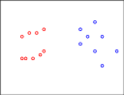Okay, this is already looking funky. Let's make it even worse. Let's apply consistency again and start moving some blue points:
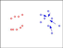Again, let's organize these into a line:
And if I had given you this data to start with, my guess is the clustering you'd have come up with is more like:
This is a violation of consistency.

So, what I'd like someone to do is to argue to my why consistency is actually a desirable property.

I can come up with lots of other examples. One reason why this invariance is bad is because it renders the notion of "reference sizes" irrelevant. This is of course a problem if you have prior knowledge (eg., one thing measured in millimeters, the other in kilometers). But even in the case where you don't know knowledge, what you can do is take the following. Take data generated by thousands of well separated Gaussians, so that the clearly right thing to do is have one cluster per Gaussian. Now, for each of these clusters except for one, shrink them down to single points. This is possible by consistency. Now, your data basically looks like thousands-1 of clusters with zero inter-cluster distances and then one cluster that's spread out. But now it seems that the reasonable thing is to put each data point that was in this old cluster into its own cluster, essentially because I feel like the other data shows you what clusters should look like. If you're not happy with this, apply scaling and push these points out super far from each other. (I don't think this example is as compelling as the one I drew in pictures, but I still think it's reasonable.

Now, in the UAI paper this year, they show that if you fix the number of clusters, these axioms are now consistent. (Perhaps this has to do with the fact that all of my "weird" examples change the number of clusters -- though frankly I don't think this is necessary... I probably could have arranged it so that the resulting green and blue clusters look like a single line that maybe should just be one cluster by itself.) But I still feel like consistency isn't even something we want.

(Thanks to the algorithms group at Utah for discussions related to some of these issues.)

UPDATE 20 JUNE 2009, 3:49PM EST

Here's some data to justify the "bad things happen even when the number of clusters stays the same" claim.

Start with this data:


Now, move some points toward the middle (note they have to spread to the side a bit so as not to decrease intra-cluster distances).

Yielding data like the following:

Now, I feel like two horizontal clusters are most natural here. But you may disagree. What if I add some more data (ie., this is data that would have been in the original data set too, where it clearly would have been a third cluster):

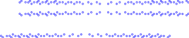
And if you still disagree, well then I guess that's fine. But what if there were hundreds of other clusters like that.

I guess the thing that bugs me is that I seem to like clusters that have similar structures. Even if some of these bars were rotated arbitrarily (or, preferably, in an axis-aligned manner), I would still feel like there's some information getting shared across the clusters.

The importance of input representations

As some of you know, I run a (machine learning) reading group every semester. This summer we're doing "assorted" topics, which basically means students pick a few papers from the past 24 months that are related and present on them. The week before I went out of town, we read two papers about inferring features from raw data; one was a deep learning approach; the other was more Bayesian. (As a total aside, I found it funny that in the latter paper they talk a lot about trying to find independent features, but in all cog sci papers I've seen where humans list features of objects/categories, they're highly dependent: eg., "has fur" and "barks" are reasonable features that humans like to produce that are very much not independent. In general, I tend to think that modeling things as explicitly dependent is a good idea.)

Papers like this love to use vision examples, I guess because we actually have some understanding of how the visual cortex words (from a neuroscience perspective), which we sorely lack for language (it seems much more complicated). They also love to start with pixel representations; perhaps this is neurologically motivated: I don't really know. But I find it kind of funny, primarily because there's a ton of information hard wired into the pixel representation. Why not feed .jpg and .png files directly into your system?

On the language side, an analogy is the bag of words representation. Yes, it's simple. But only simple if you know the language. If I handed you a bunch of text files in Arabic (suppose you'd never done any Arabic NLP) and asked you to make a bag of words, what would you do? What about Chinese? There, it's well known that word segmentation is hard. There's already a huge amount of information in a bag of words format.

The question is: does it matter?

Here's an experiment I did. I took the twenty newsgroups data (standard train/test split) and made classification data. To make the classification data, I took a posting, fed it through a module "X". "X" produced a sequence of tokens. I then extract n-gram features over these tokens and throw out anything that appears less than ten times. I then train a multiclass SVM on these (using libsvm). The only thing that varies in this setup is what "X" does. Here are four "X"s that I tried:

1. Extract words. When composed with extracting n-gram tokens, this leads to a bag of words, bag of bigrams, bag of trigrams, etc., representation.
2. Extract characters. This leads to character unigrams, character bigrams, etc.
3. Extract bits from characters. That is, represent each character in its 8 bit ascii form and extract a sequence of zeros and ones.
4. Extract bits from a gzipped version of the posting. This is the same as (3), but before extracting the data, we gzip the file.

The average word length for me is 3.55 characters, so a character ngram with length 4.5 is approximately equivalent to a bag of words model. I've plotted the results below for everything except words (words were boring: BOW got 79% accuracy, going to higher ngram length hurt by 2-3%). The x-axis is number of bits, so the unigram character model starts out at eight bits. The y-axis is accuracy:
As we can see, characters do well, even at the same bit sizes. Basically you get a ton of binary sequence features from raw bits that are just confusing the classifier. Zipped bits do markedly worse than raw bits. The reason the bit-based models don't extend further is because it started taking gigantic amounts of memory (more than my poor 32gb machine could handle) to process and train on those files. But 40 bits is about five characters, which is just over a word, so in theory the 40 bit models have the same information that the bag of words model (at 79% accuracy) has.

So yes, it does seem that the input representation matters. This isn't shocking, but I've never seen anyone actually try something like this before.